Measuring the speed of sound

If we look at the original data points again, we can make out a couple of points that don’t seem to belong to the others. We seem to have a few outliers:

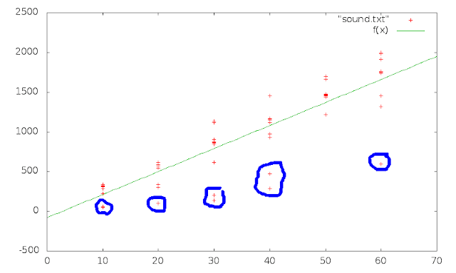
This is a kinda subjective decision, but I hope you agree that those points close to 0 at 10, 20 and 30 cm don’t make any sense and that the ones at 40 and 60 cm seem to be too far away from the other points at that distance to actually belong to them. My guess is that I messed up the clapping for those points and that start and/or stop were caused by some reflection of the walls and furniture rather than the direct sound wave source -> mic A -> mic B.

This is a touchy issue and while this measurement of the speed of sound doesn’t matter and the value of the actual result we get has no consequences whatsoever, this is not true for proper, publicly funded science. There, a lot of money and reputation could be at stake or even human lives. Whenever you have to tamper with your data, you should make 100% sure that you’re doing it to get closer to the truth and NOT to the result you’d like to see.

A good way to make sure that you don’t influence the result to your own liking (be it consciously or subconsciously) is to decide what kind of data to cut away before looking at the actual data. This is called a blind study and was, for example, done for the discovery of the (probably) Higgs boson. The scientists at CERN didn’t actually look at the interesting part of the data until they had their analysis fixed. Before that they were only looking at the data left and right of the interesting part, to test their programs and tweak the cuts.

And whatever you do, if you do something to the data, you DO NOT do it in secrecy. If you cut away data, show it and tell the world (or at least the other 5 people that read your paper) why you chose to do so and what it achieved. Science is all about openness and getting closer to the truth together, not trying to prove your point.

Anyway, if we remove those outliers from our data (just add a ‘#’ to the beginning of the corresponding lines in the data file and loadtxt will ignore them), our results again change a little bit:

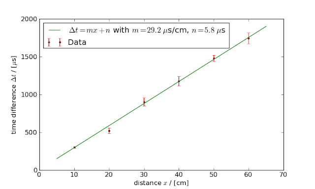
Now we reached an (estimated) accuracy of 2.6%. Not too bad for an afternoon measurement! (Writing up this article has taken way more time than producing the actual results.)

To summarize: from the naive idea of “just” measuring the time and distance of sound travelling from a source to a microphone, we developed a strategy to measure the speed of sound with minimal systematic errors. We then did the measurement and gradually improved the accuracy of our measurement by improving the data analysis. Note that each improvement of accuracy is actually compatible with the results before. Every result lies within one sigma (i.e. one standard deviation) of the previous results. This means that all of our results are equally true, as long as you consider their uncertainties. If you compare our result with the values given at Wikipedia they also are very compatible. (The temperature at the time of the measurement was around 18°C according to the weather forecast.) Yes, I know, never quote Wikipedia in a scientific work, but it’s pretty convenient to quickly look up something.

Phew, this article turned out way longer than I intended it to be.

tl;dr: Science works! 😉

See you around…

Pages: 1 2 3 4

• experiment
• physics
• speed of sound